Density-based clustering algorithm is an unsupervised machine learning clustering algorithm that detects areas of high density and low density. Including time is one of the important aspects of any clustering algorithm. ArcGIS Pro’s Density-based Clustering Tool allows users to apply the clustering algorithm both in the space and time paradigm.
The Density-based Clustering tool’s Clustering Methods parameter provides three options:
- Defined distance (DBSCAN)
- Self-adjusting (HDBSCAN)
- Multi-scale (OPTICS)
In the current blog, we will explain and highlight key points of Defined distance (DBSCAN). This algorithm requires the user to have a clear Search Distance. It also allows the user to use the Time Field and Search Time Interval parameters to find clusters of points in space and time.
How it works
DBSCAN – defined distance with time, finds clusters of point features based on their spatial distribution. In the high-density region, the algorithm identifies groups as clusters and low-density regions are left as noise. Inclusion of time in this analysis will create space-time clusters.
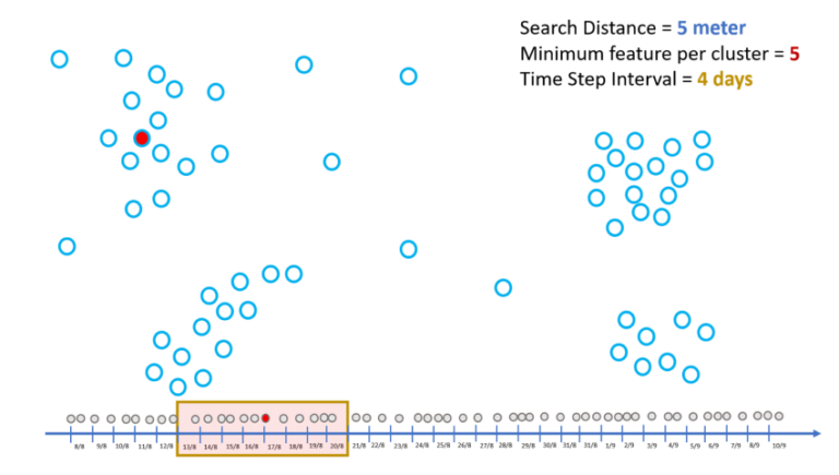
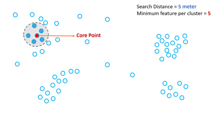
To define high-density and low-density regions, two parameters are considered. One being Search Distance and the other being Minimum feature per cluster. If two parameters are met then that region will be a high-density region and those regions which do not meet these two criteria, will be low density regions.
Within the high-density region, the algorithm chooses a point of interest and then scans for the given Search Distance for a given number of Minimum features. If the algorithm succeeds with the point of interest, then the point becomes Core Point and the cluster is defined for that Core Point.
How Does the Cluster Grow?
To grow the existing cluster, the algorithm chooses one of the neighbors in the cluster associated with Core Point. It then scans the neighboring space for two same parameters. If the criteria are met, then the chosen neighbor will be the new Core Point. Chosen neighbor along with its neighbors become part of a growing cluster.
If criteria are not met, then it becomes Boundary Point and the cluster will not grow beyond the Boundary Point. The points which are neither boundary points nor core points will not be part of the growing clusters. These points are made part of a low-density area and hence Noise. The algorithm does this activity for every point thereby identifying Core Points and Boundary Points. The combination of Core Points and Boundary Points gives clusters.
When time is added to the clustering algorithm, output clusters become more sensitive to the time. This will refine the result. This refinement comes with redefining the neighborhood. With the inclusion of time, neighbors of Core Points are not just spatial neighbors, but they should also be temporal neighbors.
Temporal neighbors are those points that are before and after the time of the Core Point. This is defined in terms of Time Step Interval. Defining Time Step Interval refines the total number of neighbors available around the Core Point. The points, which are not spatial and temporal neighbors, are left out from the analysis. Once this refinement is done; the clustering algorithm builds clusters around the Core Point and those that are not the part of the cluster are pushed out as Noise. With the above basic understanding of how Density-based Clustering Tool works, let us use the tool to understand where habitat clusters of Malabar Pied-Horbill exist in India.
-
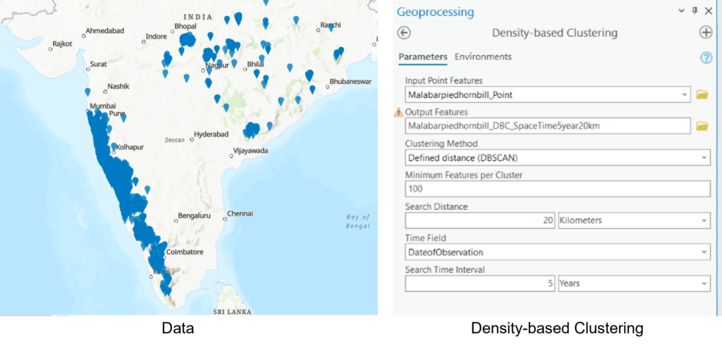
Figure 1 : Data and ArcGIS Pro’s Density-based Clustering Tool
Finding Malabar Pied-Hornbill Clusters
Malabar Pied-Hornbill is a majestic bird that is spread all along western ghats and some parts of the Vindhya mountains. Data related to various observations of this majestic bird has been meticulously documented and is being shared via Global Biodiversity Information Facility (https://www.gbif.org/dataset/search). We have downloaded historic data (shown below in Figure 1.a) of bird observation with the objective of finding spatio-temporal clusters.
For identifying spatio-temporal clusters, we have used ArcGIS Pro’s Density-based Clustering tool (as shown above in Figure 1.b) with Defined distance (DBSCAN) as the clustering method. We also defined other parameters like Minimum Feature per Cluster (100 in this case), Search Distance (20 Kilometers) and Search Time Interval (5 years).
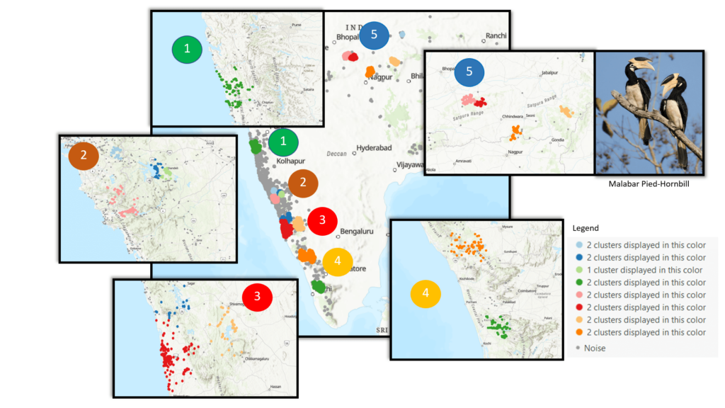
Resulting clustering contains 15 clusters spread across 5 regions. These regions (as shown in Figure 2) are
- Region 1: Coastal Maharashtra
- Region 2: Goa and Coastal Karnataka
- Region 3: Western Ghats of Karnataka
- Region 4: Kerala Region
- Region 5: Nagpur Region
Using Density-based Clustering tool, we were able to answer some of the toughest questions of ecology with the click of a button. We were able to answer whether there exist spatio-temporal clusters (in the Malabar Pied-Hornbill dataset) or not? If clusters exist, then how many clusters exist and where these are spread across? Answering such questions is key for any policy level decision related to conservation of species.
Key Takeaway
Clustering tools are used to identify spatio-temporal clusters in the data related to events, like bird observation, accidents, theft incidents etc. Identifying clusters gives definitive direction for the policy makers or analysts working on pattern recognition. In the case of Malabar Pied-Hornbill, the results could be used for a concentrated and hyper local conservation effort keeping clustered area in focus.

I am an Assistant Manager on the Presales team designing India-specific GIS solutions for our customers.