Landsat based detection of Trends in Disturbance and Recovery (LandTrendr) is one of the few ways of analyzing disturbance in vegetation using a time series of satellite imagery in ArcGIS Pro. LandTrendr algorithm analyses each pixel in the series and brings out spectral trajectories of land surface change from yearly Landsat time-series. This can also be performed on Landsat based indices like NBR, NDVI, NDSI or NDBI etc.
LandTrendr Model
The objective is to access disturbance patterns across the landscape through a series of Landsat images. This vegetation disturbance could be because of logging, disease, or forest fire. To achieve this objective, we have used a new, easy to use GP tool called Analyze Changes using LandTrendr.
What can LandTrendr Model answer?
LandTrendr helps you to answer the following questions using a stack of images collected over time:
- Has anything changed? When did the change start, and how long did it last?
- Was the change in the positive direction (e.g. forest recovery) or negative direction (e.g. forest disturbance)?
- Was it a slow change (e.g. plant regrowth) or an abrupt change (logging or fire)?
- How many such changes occurred within a defined period?
- How does LandTrendr work?
LandTrendr algorithm is based on segmentation of pixel value trajectories over time. In the model, each pixel value is graphed over time and fitted with a linear model. The different line segments indicate various parts of the pixel’s change story. This understanding has been captured in Figure 1 where a linear model is fitted to a single pixel’s values over time. There are points, which have steep changes, have negative changes, a longer, and a slower positive change.
The output from the LandTrendr tool is a change analysis raster, and it contains model information like the start and end date of changes along with change duration and magnitude.
Chikkamangaluru District Case
We have chosen Chikkamangaluru district as the study area. 63 cloud free spring season Landsat images spanning over 30 years (1990 to 2020) were downloaded. On average two images have been taken for each season.
To analyze the forest disturbance, an index-based approach is quite efficient. For LandTrendr, any single band index (that represents vegetation) can be used. In our study, we have used NBR i.e. Normalized Burned Ratio. The NBR formula is similar to NDVI, except that the formula combines vegetation sensitive bands i.e. near infrared (NIR) and shortwave infrared (SWIR).
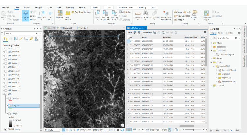
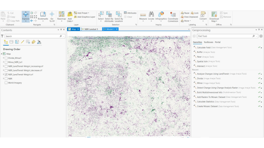
For the current study, NBR was calculated for all 63 Landsat images. Each of these were added to a mosaic dataset. It should be noted that NBRs should have a date component in one of the columns. This date should be the date of acquisition of the Landsat image. All this data preparation activity was done on ArcGIS Pro (as shown in the below image).
Once the NBR Mosaic Dataset was produced, we used a geoprocessing tool called Analyze Changes Using LandTrendr. All default values were kept for running this tool on NBR Mosaic Dataset. Output was a Cloud Raster Format (CRF) multidimensional raster dataset (Figure 3) containing model information from the LandTrendr analysis.
-
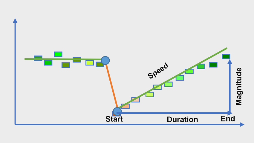
Figure 1 : Working of LandTrendr
Results
Change analysis raster contains the model coefficients. This modelled FittedValue is included in the output as a band. This provides the pixel value when it is fitted to the modeled line segment at that point in time.
Though model coefficients are difficult to interpret visually, there are additional tools to use to interpret the data. Temporal profile chart can be created to explore pixel changes over time, using the FittedValue band. Changes that have happened over years can be seen in the temporal graph. For example (as in Figure 4), there are 4 changes marked as Change 1, Change 2, Change 3 and Change 4.
Discussion
In this discussion part, we will be looking into a few points and their temporal behavior using the output of Analyze Changes Using LandTrendr. Let us check 3 locations to understand different scenario.
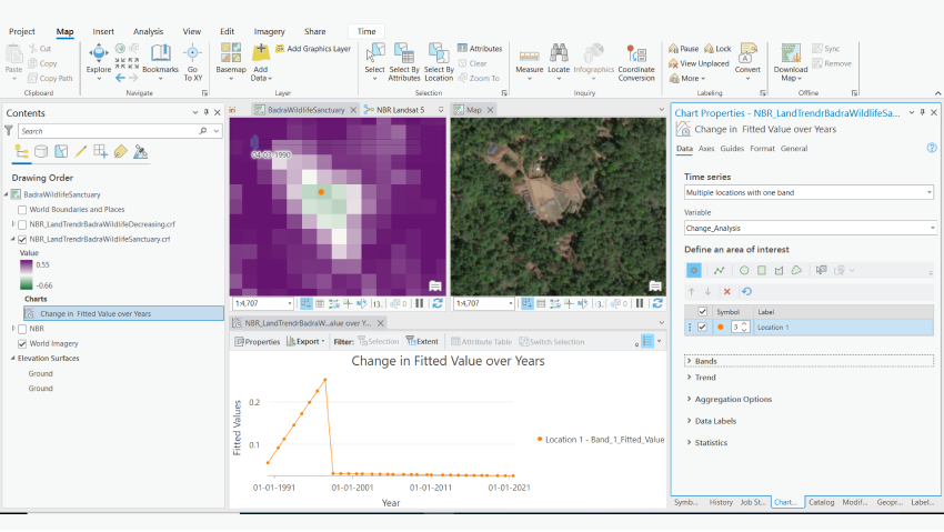
Location 1 (Refer to Figure 6): This location is near Chikkamagaluru city. On click, you will see the graph showing an abrupt decrease in 1997. After 1997, it never recovered back. This is typical case of land clearance.
Location 2 (Refer to Figure 7): Now let us explore another location which is at the fringes of the forest. The graph shows gradual increase and then abrupt decrease in NBR followed by increase. This is typical of a forest fire scenario. We have this situation in 2013. Vegetation started improving after 2016.
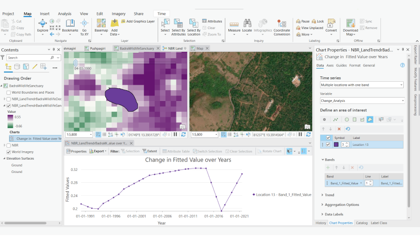
Location 3 (Refer to Figure 8): Temporal Profile tool also has option to analyze using AOI. We used free hand to draw AOI and see when a disturbance had happened. From the graph, the disturbance started before 1991 and there is a gradual decrease. It became low by 2001 and slowly recovered by 2014. This type of scenario is typical of disease infestation and recovery.
-
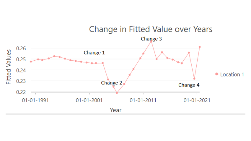
Figure 4 : Temporal Graph of FittedValue
Like the above 3 scenarios, we can assess a given area using the LandTrendr model for finding land cover disturbances. LandTrendr model can also be used to assess lake disappearances in the urban scenario, forest-agriculture landuse change etc. LandTrendr, though a data intensive model, is a crucial one when it comes to identifying and understanding land cover disturbances using Landsat data.

I am an Assistant Manager on the Presales team designing India-specific GIS solutions for our customers.